Search for New Physics.
Most recent reference:
M. Bona et al. [UTfit Collaboration], "The UTfit Collaboration Report on the
Unitarity Triangle beyond the Standard Model: Spring 2006"
hep-ph/0605213
Generalization of UT analysis beyond the SM:
Results for
Universal Unitarity Triangle analysis and Minimal Flavour Violation scenario
Model Independent Approach to |ΔF|=2 Hamiltonian
Starting from the New Physics Free determination
of ρ and η,
we explore, in a model-independent approach, the possible contributions of
NP effects to Bd-Bd,
Bs-Bs and
K0-K0 mixing.
Each of these processes can be parameterized in terms of only two new parameters, which we
choose to quantify the difference of the amplitude, in absolute value and phase,
with respect to the SM one. Thus in the case of
Bq-Bq mixings,
we define
|
CBq e2 i φBq =
|
|
(q=d,s)
|
|
=
|
|
AqSM e2iφqSM+
AqNP e2i(φqNP+φqSM)
|
|
(q=d,s)
|
|
where HeffSM includes only the SM box diagram,
while Hefffull includes also the NP contributions.
In the second equation we also introduce φqSM
where φdSM = β and φsSM = -βs
These definitions imply that the mass differences and the CP asymmetry
are related to the SM counterparts by
|
Δmd=CBd ⋅ ΔmdSM
|
|
Δms=CBs ⋅ ΔmsSM
|
|
βexp = βSM + φBd
|
|
αexp = αSM - φBd
|
|
βsexp = βsSM - φBs
|
Concerning K0-K0 mixing, we
introduce a single parameter which relates the imaginary part of the amplitude to the SM one,
This definition implies a simple relation for |εK|:
While in the previous analyses (Winter 2006) we could not consider the full case of
CBs for being Δ ms not yet measured,
recent experimental developments are now allowing for dramatic improvements in the
Bs sector together with improved measurements in the Bd sector:
These constraints allow for a complete NP analysis with the fully model-independent
determination of CKM parameters ρ
and η, obtaining simultaneously
predictions on all the NP quantities introduced above.
In the general model-independent analysis we also have to consider Δ F = 1
effects: below are the detailed descriptions of the various constraint treatments.
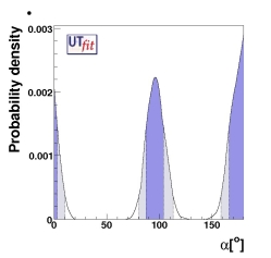
α and New physics in |&Delta F|=1
In principle, the extraction of α from B → ππ, ρπ, and
ρρ decays is affected by NP effects in |Δ F|=1 transitions.
In the presence of NP in the strong b &rarr d penguins, the decay
amplitudes for B mesons decaying into ππ, ρπ, and ρρ
are a simple generalization of the SM ones (given for example
here):
Assuming that NP modifies significantly only the "penguin" amplitude P
without changing its isospin quantum numbers (i.e. barring large isospin-breaking
NP effects), the only necessary modification amounts to distinguish the
penguin complex parameters P and
P, which
come from the sum of SM and NP contributions in B and
B decays and which bring in general
different weak and strong phases.
The procedure to extract α is the same as in the
SM case but the expected bound is weaker
due to the presence of two (four) extra parameter(s) for ππ and ρρ
(ρπ).
Since NP effects in |ΔF|=2 are not included, this constraint has to be
interpreted as a bound to α-φBd
(see above) once it is used in the extension of the UT analysis including
NP in |ΔF|=2.
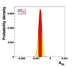
Semi-leptonic Asymmetry ASL and New Physics effects
One can also add the constraint coming from the CP asymmetry in semi-leptonic B decays
ASL, defined as
|
ASL =
|
|
Γ(B0 → l+X) -
Γ(B0 → l-X)
|
|
Γ(B0 → l+X) +
Γ(B0 → l-X)
|
|
|
It has been noted in hep-ph/0202010
that ASL is a crucial ingredient of the UT analysis once the formulae are
generalized as described below, since it depends on both CBd and
φBd. Infact, we can write:
|
ASL = - Re(Γ12/M12)SM
|
|
+ Im(Γ12/M12)SM
|
|
|
where Γ12 and M12 are the absorptive and
dispersive parts of the
B0d-B0d
mixing amplitude.
At the leading order, ASL is independent of penguin operators,
but, at the NLO, the penguin contribution should be taken into
account. In the SM, the effect of penguin operators is GIM suppressed
since their CKM factor is aligned with M12: both are proportional
to (V*tbVtd)2. This is not true anymore
in the presence of NP, so that the effects of penguins are amplified beyond
the SM. We therefore start from the full NLO calculation of
hep-ph/0308029, allowing
for an additional NP contribution to the penguin term in the |Δ F |=1
amplitude. This introduces two additional parameters CPen
and φPen that, because of the extra
αs factor, enter as a smearing in the expression of
ASL. The generalized expression of ASL is given in
hep-ph/0509219
BaBar has recently released a new improved
ASL measurement that in association with the quantity ACH
described in the following allows for further constraining the φBd
and CBd; NP parameters. As can be seen below, the actual
measurements of these two observables strongly disfavour the solution with
ρ and
η in the third quadrant,
which now has only 0.4% probability.
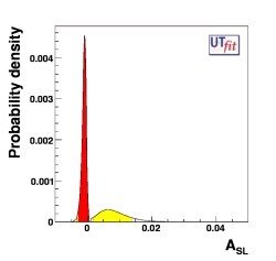
Here we show the one-dimensional distributions for this quantity both in the
Standard Model fit (left plot)
and in the New Physics general scenario (right plot).
See the table for the numerical results.
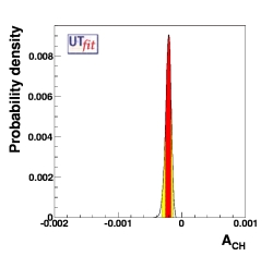
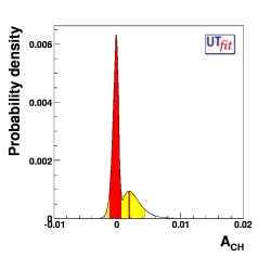
Dimuon Charge Asymmetry ACH
The charge asymmetry ACH in dimuon events is a rather unique constraint
since it depends on ρ and
η and on all ΔB=2 NP parameters
(CBd, φBd, CBs, and
φBs). D0 Collaboration has recently announced a
new result
for this observable. The dimuon charge asymmetry ACH can be defined as:
|
ACH =
|
|
|
=
|
|
ξ(P1+P3)+(1-ξ)P2+0.28P7+0.5P'8+0.69P13
|
|
|
using the notation as in the D0 result
where the definition and the measured values for the P parameters can be found. We have:
|
χ = fdχd+fsχs;
|
|
χ =
fdχd+
fsχs;
|
|
ξ = χ + χ
- 2 χχ;
|
where we have assumed equal semi-leptonic widths for Bd andn Bs
mesons, fd = 0.397 ± 0.010 and fs = 0.107 ± 0.011
are the production fractions of Bd and Bs mesons respectively
and the χq and χq
are given in equation 6 in .
They contain the dependence (through equations 7 in the same ref.) on the ΔB=2 NP parameters
(CBd, φBd, CBs, and
φBs) as well as the possible NP contributions to ΔB=1
penguins (CqPen, φqPen).
Here we show the one-dimensional distributions for this quantity both in the
Standard Model fit (left plot)
and in the New Physics general scenario (right plot)
See the table for the numerical results.
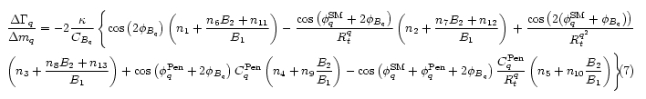
Width Difference ΔΓq
In presence of New Physics, the measurement of ΔΓq is
related to ρ
and η, and to the NP
parameters CBq and φBq
through the value of Δmq: you can find the relation
here (eq. 7 in
hep-ph/0605213)
A simultaneous use of Δmq and of the bound from
ΔΓq allows to constrain the phase of the mixing even
without a direct measurement of the mixing phase.
This is particularly important in the case of the Bs sector,
waiting for the measurement on the time-dependent CP asymmetry in
Bs → J/ψ φ
Since the available experimental measurements are not directly sensitive to
the phase of the mixing amplitude, they are actually a measurement of
&Delta&Gammaq cos2(φBq- βq)
in the presence of NP.
Predictions for Semi-leptonic and Dimuon Charge Asymmetries in SM and in NP scenarios
We add here the prediction on the quantities previously described:
ASL, ACH, ΔΓq/Γq.
These are obtained from the fully model-independent fit without using
the given quantities. The values represent the allowed ranges in this generalized
framework. For comparison also the SM values are given together with the experimental
measurements.
|
Results of NP generalized analysis
|
|
Parameter
|
Solution in SM scenario
|
Solution in NP analysis
|
Experimental Measurements
|
|
103ASL
|
-0.71 ± 0.12 |
[-3.3, 13.8] @95% Prob. |
-0.3 ± 5.0 |
|
103ACH
|
-0.23 ± 0.05 |
[-1.6, 4.8] @95% Prob. |
-1.3 ± 1.2 ± 0.8 |
|
103 ΔΓd/Γd
|
3.3 ± 1.9 |
2.0 ± 1.8 |
9 ± 37 |
|
ΔΓs/Γs
|
0.10 ± 0.06 |
0.00 ± 0.08 |
0.25 ± 0.09 |
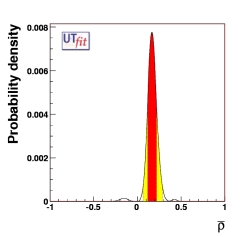
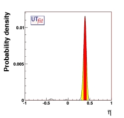
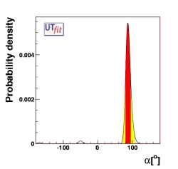
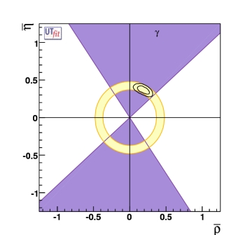
UT parameters
We list below the result of the fully model-independent fit in terms of UT quantities
including possible NP contributions as described above. These values represent
the allowed ranges in this generalized framework. We found only one favoured solution,
corresponding to the result of the Standard Model fit, while the second region,
corresponding to the UT with its vertex in the third quadrant and implying sizable
New Physics effects in the Bd sector, present in the
previous version of
this analysis is now excluded at 95% probability.
|
Results of NP generalized analysis
|
|
Parameter
|
68% probability Region
|
|
ρ
|
0.169 ± 0.051 |
|
η
|
0.391 ± 0.035 |
|
α
|
(88 ± 7)o |
|
β
|
(25.1 ± 1.9)o |
|
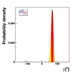
γ
|
(67 ± 7)o |
|
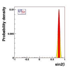
sin2β
|
0.771 ± 0.040 |
|
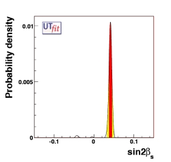
sin2βs
|
0.042 ± 0.004 |
|
105 Im λt
|
15.6 ± 1.3 |
|
103 Re λt
|
-0.315 ± 0.020 |
|
103|Vub|
|
4.12 ± 0.25 |
|
102|Vcb|
|
4.15 ± 0.07 |
|
103|Vtd|
|
8.62 ± 0.53 |
|
Vtd/Vts|
|
0.211 ± 0.013 |
|
Rb
|
0.428 ± 0.027 |
|
Rt
|
0.921 ± 0.055 |
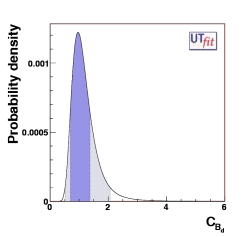
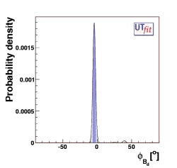
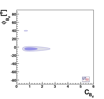
New Physics in Bd-Bd mixing
Because of the abundance of experimental information, one can determine
stringent bounds to NP parameters, simultaneously to the determination of
the UT parameters given above. The following plots show what we obtain for
CBd and φBd.
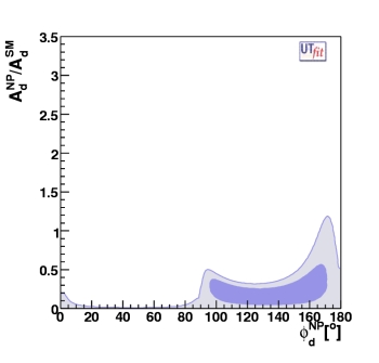
We can also write
|
CBq e2iφBq =
|
|
AqSMe2iβ
+ AqNPe2i(β+φqNP)
|
|
|
and given the p.d.f. for CBd and
φBd, we can derive the
p.d.f. in the (ANP/ASM) vs
φNP plane.
The result is shown in the figure above on the right.
We see that the NP contribution can be substantial if its phase is close to
the SM phase, while for arbitrary phases its magnitude has to be much
smaller than the SM one. Notice that, with the latest data, the SM
(φBd=0) is disfavoured at 68% probability due to
a slight disagreement between sin 2β and |Vub/Vcb|.
This requires ANP ≠ 0 and φNP ≠ 0. For the
same reason, φNP > 90o at 68% probability and the
plot is not symmetric around φNP = 90o.
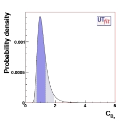
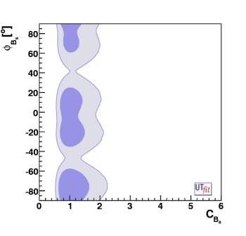
New Physics in Bs-Bs sector
Because of the abundance of experimental information, one can determine
stringent bounds on NP parameters, simultaneously with the determination of
the UT parameters and the Bd-related NP parameters given above.
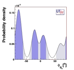
The following plot shows what we obtain for CBs and
φBs.
Thanks to the good precision of the new
new Δms measurement
and the good precision on ξ from lattice QCD, the bound on
CBs is already more precise than the bound on
CBd. Also the ACH and ΔΓs
measurements can now provide the first constraints on φBs.
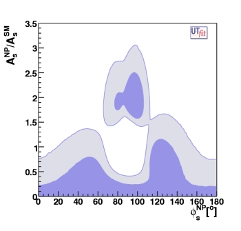
As in the case above of the Bd-Bd
mixing, we can define in the same way AsNP/AsSM and
φsNP as functions of CBs and
φBs
and given the p.d.f. for CBs and
φBs, we can derive the
p.d.f. in the (AsNP/AsSM) vs
φNP plane.
The result is shown in the figure above on the right and we have exclusion regions for the first
time, thanks to the new measurements described above (ACH and Δ&Gammas).
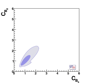
Correlation in the New Physics between Bd and Bs sectors
We'd like to point out an interesting correlation between the values of CBd
and CBs that can be seen in the figure below. This correlation that is
present in the general analysis, is due to the fact that lattice QCD determines quite precisely
the ratio ξ2 of the matrix elements entering Bd and Bs
mixing amplitudes.
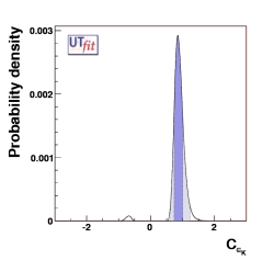
New Physics in K0-K0 sector
Because of the abundance of experimental information, one can determine
stringent bounds on NP parameters, simultaneously with the determination of
the UT parameters and the Bd-related NP parameters given above.
The following plot shows what we obtain for CεK.
Universal Unitarity Triangle and Minimal Flavour Violation
It is possible to generalize the full UTfit beyond
the Standard Model to all those NP models characterized by Minimal Flavour Violation, i.e.
having quark miking ruled only by the Standard Model CKM couplings. In fact, in this case no
additional weak phases are generated and several observables entering into the Standard Model
fit (the tree-level processes and the measurement of angles through the use of time
dependent CP asymmetries) are not affected by the presence of New Physics. The only sizable
effect we are sensitive to is a shift of the Inami-Lim function of the top contribution
in meson mixing. This means that in general εK and Δmd cannot be used
in a common SM and MFV framework, but any New Physics contribution disappear in the case of
Δmd/Δms. So, simply removing the information related to
εK and Δmd from the full UTfit one can obtain a more precise determination
of the Universal Unitarity Triangle,
which is a common starting point for the
Standard Model and any MFV model.

(EPS)
[JPG]
ρ = 0.153 ± 0.030
from UUT fit
|

(EPS)
[JPG]
η = 0.347 ± 0.018
from UUT fit
|

(EPS)
[JPG]
PREDICTIONS:
α = (91.3 ± 4.8)o
from UUT fit
|

(EPS)
[JPG]
PREDICTIONS:
β = (22.3 ± 0.9)o
from UUT fit
|

(EPS)
[JPG]
PREDICTIONS:
γ = (66.3 ± 4.8)o
from UUT fit
|

(EPS)
[JPG]
PREDICTIONS:
sin2βs = 0.037 ± 0.002
from UUT fit
|
One has to notice that the precision on ρ and
η is in practise the same than in the full UTfit.
This means that one can go forward in the study of MFV,
using the two neglected informations
(εK and Δmd) to bound the scale of New Physics. In fact, the expected
contribution is a shift of S0, the Inami-Lim function associated to top contribution
in box diagrams. The shift can than we translated in terms of the tested energy scale for
New Particles, using a simple dimensional argument.
where δS0 is the shift, a is a parameter related to Wilson coefficients of the effective
Hamiltonian, Λ is the New Physics scale and
Λ0=Ytsin2(θW)MW/α ∼ 2.4 TeV is the reference
EW scale. One can extract Λ0 in two different scenarios:
- MFV models with one Higgs doublet or low/moderate tanβ. In this case, the shift δS0 is
a universal factor for all the mixing processes we are considering
(K0-K0,
B0-B0, and
Bs-Bs).
The information coming from those mixing processes that are ignored in UUT can be used to
bound this universal shift, once the CKM parameters are fixed by the UUT.
- MFV models with large values of tanβ. In this case, it is still true that one can
use εK and Δmd to bound the New Physics shift. But, in this case,
one cannot simply relate the effect on
K0-K0
to the corresponding quantity in B physics (which remains common to
B0-B0 and
Bs-Bs).
Here we show the result in terms of the output distribution of δS0 (δS0B
and δS0K) in the case of models with low/moderate (large) values of tanβ
and we give the output value in terms of the tested energy scales, quantified at the 95% Probability.

(EPS)
[JPG]
δS0 = -0.16 ± 0.32
|

(EPS)
[JPG]
δS0B = 0.05 ± 0.67
|

(EPS)
[JPG]
δS0K = -0.18 ± 0.37
|
Λ > 5.5 TeV @95% Prob.
for small tanβ
|
Λ > 5.1 TeV @95% Prob.
for large tanβ
|


 plane")
![[JPG]](NPalpha.jpg)
![[JPG]](ASL_dSM.jpg)
![[JPG]](ASL_dNP.jpg)
![[JPG]](ACH_SM.jpg)
![[JPG]](ACH_NP.jpg)
![[JPG]](NP-rho.jpg)
![[JPG]](NP-eta.jpg)
![[JPG]](NP-alpha.jpg)
![[JPG]](NP-beta.jpg)
![[JPG]](NP-gamma.jpg)
![[JPG]](NP-sin2bs.jpg)
![[JPG]](NP-rhovseta.jpg)
![[JPG]](C_BdNP.jpg)
![[JPG]](Phi_BdNP.jpg)
![[JPG]](cvsphi-np.jpg)
![[JPG]](achilleplot.jpg)
![[JPG]](C_BsNP.jpg)
![[JPG]](Phi_BsNP.jpg)
![[JPG]](cbsvsphibs-np.jpg)
![[JPG]](achilleplot_Bs.jpg)
![[JPG]](cbdvscbs.jpg)
![[JPG]](C_epsKNP.jpg)
![[JPG]](uut.jpg)
![[JPG]](UUT_rho.jpg)
![[JPG]](UUT_eta.jpg)
![[JPG]](UUT_alpha.jpg)
![[JPG]](UUT_beta.jpg)
![[JPG]](UUT_gamma.jpg)
![[JPG]](UUT_sin2bs.jpg)
![[JPG]](deltaS0.jpg)
![[JPG]](deltaS0_B.jpg)
![[JPG]](deltaS0_K.jpg)