The decay amplitudes B → π⁺π^- and B → ρ⁺ρ^- are characterized by two different CKM terms: the favored term V_tb^*V_td, which multiplies a pure penguin amplitude (sometimes called P), and the suppressed term V_ub^*V_ud, which multiplies the sum of tree, penguin and annihilation contributions (sometimes called T, since the tree part is expected to be dominant). Since the weak phase γ enters into the suppressed amplitude, in a scenario of tree contribution dominance a time dependent analysis of the CP asymmetry

in these decays allows a measurement of the angle sin(2α) from the value of the coefficient S of the sine term in the oscillation and the use of the unitarity of CKM matrix.

Since the tree dominance is just a naive approximation of the actual dynamic, what one can really measure from S is sin(2α_eff), where 2α_eff = 2α+ κ (κ being the relative strong phase between T and P amplitudes). The extraction of α from α_eff is model dependent, since there is no way to access directly κ. From a theoretical point of view, the cleanest method now available is the isospin analysis, originally proposed by M. Gronau and D. London. Starting from the measurement of all BR and CP asymmetries of ππ (ρρ) decays, one can build two triangles

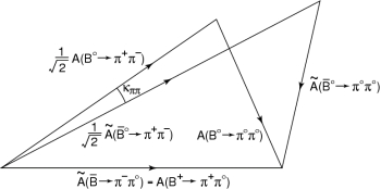
which, in the limit of exact isospin symmetry, have a side in common and are tilted by the angle κ. This approach has two main problems:

• The determination of α comes with ambiguity related to trigonometric relations. See L. Ross's contribution to the Second CKM Workshop for details.
• Isospin breaking effects are neglected. Possible contributions to the breaking come from EW penguin diagrams and possible FSI effects. For a recent on this subject, see M. Ciuchini's talk at the first BaBar CKM Angles Physics Workshop

Moreover, the time dependent analysis of (ρπ)⁰ final state on the Dalitz plot provides additional information on α. In particular, thanks to the fact that a Dalitz analysis allows to extract absolute value and phases for the tagged decay amplitude, it is possible to cancel out the penguin contribution assuming SU(2) flavour symmetry, in a similar way than the method proposed in hep-ph/0601233 and hep-ph/0602207. In the SU(2) limit, the three decay amplitudes can be written as

where the the absolute values of the T and P complex parameters include the matrix elements and the absolute values of the CKM factors, while the phases correspond to the strong phases. Using this relation, one can write the amplitude

and, in a similar way, one can define the amplitude A for the CP conjugated process. The ratio of the two amplitudes give

and (unlike the case of the isospin analysis of B → ππ and B → ρρ) any dependence on hadronic matrix elements is eliminated, since the value of α is obtained directly from data, without any need of parameterizing the matrix elements. The BaBar and Belle collaborations reported the result of the time-dependent Dalitz analysis in terms of 26 bilinear quantities, which are functions of the six tagged decay amplitudes. One overall strong phase is arbitrary. In addition, since both the experimental observables and the R quantity are ratios (the experimental values are all given in units of the quantity U^+-₊), one absolute amplitude is arbitrary as well. We fix A(B⁰ →ρ⁺ π^-) = 1 and we take the absolute values of the other six variables in the range [0,2], while the phases are taken in the range [-π, π]. We calculate the 26 experimental observables from these values and we compute the likelihood as the product of the likelihoods by BaBar and Belle

We summarize in the table below the input values in this study. The averages of for ρρ and ππ are raken from HFAG. In the case of ρρ, S and C values refer to longitudinally polarized events. The fraction of longitudinally polarized events, f_L, is also quoted.

The isospin construction described above has eight possible solutions, which nowdays cannot be distinguished unless unphysically small values of C.L. are taken into account. Nevertheless, as discussed in hep-ph/0701204 for the case of B → π π decays, it is possible using basic properties of the hadronic matrix elements, related to the the properties of QCD, it is possible to remove some of the solutions, corresponding to infinite and strongly correlated values of the hadronic matrix elements. In particular, using the fact that different arguments suggest that the tree-level contributions are of O(1) and that, we require them to be in the range [0,10], allowing all these arguments to be wrong by more than O(1) effects. At the same time, even allowing SU(3) breaking effects as large as 100%, the measured value of BR(B_s → K⁺K^-) implies that the pennguin contribution is in the range [0,2.5]. The loose requirements we applied are strong enough to exclude the unphysical regions around α ~ 0^o and α ~ 180^o, in agreement with the observation of CP violation in B → π π decays and regardless the statistical approach used in input (moreover, has discussed in hep-ph/0701204, frequentistic and bayesian approaches give comparable results when compared at a statistically significant probability/C.L. and when the same physics inputs are used).

(EPS) [JPG] ππ Only: α = [86,167]o@ 95% Prob.	(EPS) [JPG] (ρπ)0 Only: α = [0,35]o U [56,180]o @ 95% Prob.
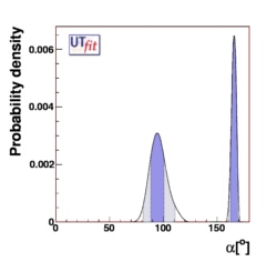
(EPS) [JPG] ρρ Only: α = [77,107]o U [160,197]o@ 95% Prob. (SM solution: α =(93 ± 10)o@ 68% Prob.)	(EPS) (JPG) ALL COMBINED: α = [81,110]o U [161,171]o@ 95% Prob. (SM solution: α =(94 ± 8)o@ 68% Prob.)

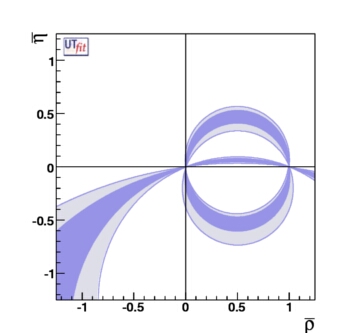
(EPS) [JPG] bound on the (ρ ; η) plane from B → ππ, B → ρρ, and and B → (ρπ)0

Observable	ππ
	Input	UTfit Output
BR(+-) (10-6)	5.2 ± 0.2	5.2 ± 0.2
BR(+0) (10-6)	5.7 ± 0.4	5.6 ± 0.4
BR(00) (10-6)	1.31 ± 0.21	1.35 ± 0.19
Observable	ρρ
	Input	UTfit Output
BR(+-) (10-6)	23.1 ± 3.3	22.9 ± 3.1
BR(+0) (10-6)	18.2 ± 3.0	15.5 ± 2.6
BR(00) (10-6)	1.16 ± 0.46	0.92 ± 0.39

(EPS) [JPG] BR+- vs BR+0 in ππ case	(EPS) [JPG] BR+- vs BR00 in ππ case
(EPS) [JPG] BR+0 vs BR00 in ππ case	(EPS) [JPG] BR+- vs BR+0 in ρρ case
(EPS) [JPG] BR+- vs BR00 in ρρ case	(EPS) [JPG] BR+0 vs BR00 in ρρ case