The impact of present Δms measurement on UT fit
Experimental Status (Winter 2006)
The CDF collaboration reported
the first 5σ measurement of Δms,
which provides a test of the Standard Model through the comparison
to the indirect determination, obtained from a combined fit to all the remaining constraints
(|Vub/Vcb|, Δ md, εK, sin2β, cos2β, α and γ).
Amplitude as a function of Δms from CDF
|
This comparison is a crucial test for the Standard Model and
it plays in the b → s sector the same role of
sin2β measurements in b → d sector few years ago. At this point,
the two informations do not show any significant evidence of disagreement
|
INDIRECT MEASUREMENT:
|
|
Pull distribution
DIRECT MEASUREMENT:
|
|
Δms = (18.4 ± 2.4) ps-1
|
|
Δms = (17.77 ± 0.12) ps-1
|
|
The amplitude method
The amplitude method has been introduced by H.G. Moser and A.Roussarie and is
described in Nucl. Instrum. Meth. A384 (1997) 491. with the aim of
setting limits on Δms and to combine results from different
analyses.
The method consists in modifying the equation describing
the probability that a B0 meson oscillates into a
B0 in the following way :
1 ± cos Δms t ⇒ 1 ± A cos Δms t.
A and σA are measured at fixed values of
Δms instead of Δms itself.
In case of a clear oscillation signal, at a given frequency, the amplitude should be
compatible with A = 1 at this frequency.
With this method it is easy to set a limit. The values of
Δms excluded at 95% C.L.
are those satisfying the condition A(Δms) +
1.645 σA (Δms) < 1.
Furthermore the sensitivity of the experiment can be defined as the value of
Δms corresponding to 1.645 σA (Δms) = 1
(taking A(Δms) = 0), namely supposing that the ``true'' value of
Δms is well above the measurable value.
For example we show, the combined result of LEP/SLD/CDF/D0 analyses (situation at Moriond06)
(see HFAG)
is shown in Figure (plot on the left) below
Amplitude as a function of Δms (HFAG WA, not including new CDF)
|
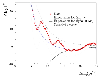
Δ log Linfinity(Δms).
|
The Likelihood ratio method
The 95% C.L. limit and the sensitivity, are useful to summarize the results of the
analysis. However to include Δms in a CKM fit and to determine
probability regions for the Unitarity Triangle parameters, continuous information
about the degree of exclusion of a given value of Δms is needed.
The log-likelihood values (it is the log-likelihood referenced to its value obtained for
Δms=infinity) can be easily deduced from A and σA using
the expressions :
 The last two equations give the average log-likelihood value for
Δms corresponding to the true oscillation frequency
(mixing case) and for Δms being far from the oscillation
frequency (|Δms-Δmstrue| >> Γ/2,
no-mixing case). Γ is here the full width at half maximum of the amplitude
distribution in case of a signal; typically Γ ~ 1/τ(Bs).
The Δ log Linfinity(Δms) plot from the world average is
shown in the above Figure (plot on the right)
The last two equations give the average log-likelihood value for
Δms corresponding to the true oscillation frequency
(mixing case) and for Δms being far from the oscillation
frequency (|Δms-Δmstrue| >> Γ/2,
no-mixing case). Γ is here the full width at half maximum of the amplitude
distribution in case of a signal; typically Γ ~ 1/τ(Bs).
The Δ log Linfinity(Δms) plot from the world average is
shown in the above Figure (plot on the right)
The Likelihood Ratio R is defined as :
 It has been shown (Yellow Book CERN-EP/2003-002
hep-ph/0304132 pages 182-190)
that in the Bayesian approach the correct method to include this information
is the Likelihood ratio method. A similar method to incorporate results from mixing can be
found in hep-ph/9607469.
It has been shown (Yellow Book CERN-EP/2003-002
hep-ph/0304132 pages 182-190)
that in the Bayesian approach the correct method to include this information
is the Likelihood ratio method. A similar method to incorporate results from mixing can be
found in hep-ph/9607469.


![[JPG]](all-DeltaMs_nodms.jpg)
![[JPG]](pull-DeltaMs_nodms.jpg)
![[JPG]](DeltaMs_direct.jpg)