The decay amplitudes B → π⁺π^- and B → ρ⁺ρ^- are characterized by two different CKM terms: the favored term V_tb^*V_td, which multiplies a pure penguin amplitude (sometimes called P), and the suppressed term V_ub^*V_ud, which multiplies the sum of tree, penguin and annihilation contributions (sometimes called T, since the tree part is expected to be dominant). Since the weak phase γ enters into the suppressed amplitude, in a scenario of tree contribution dominance a time dependent analysis of the CP asymmetry

in these decays allows a measurement of the angle sin(2α) from the value of the coefficient S of the sine term in the oscillation and the use of the unitarity of CKM matrix.

Since the tree dominance is just a naive approximation of the actual dynamic, what one can really measure from S is sin(2α_eff), where 2α_eff = 2α+ κ (κ being the relative strong phase between T and P amplitudes). The extraction of α from α_eff is model dependent, since there is no way to access directly κ. From a theoretical point of view, the cleanest method now available is the isospin analysis, originally proposed by M. Gronau and D. London. Starting from the measurement of all BR and CP asymmetries of ππ (ρρ) decays, one can build two triangles

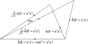
which, in the limit of exact isospin symmetry, have a side in common and are tilted by the angle κ. This approach has two main problems:

• The determination of α comes with ambiguity related to trigonometric relations. See L. Ross's contribution to the Second CKM Workshop for details.
• Isospin breaking effects are neglected. Possible contributions to the breaking come from EW penguin diagrams and possible FSI effects. For a recent on this subject, see M. Ciuchini's talk at the first BaBar CKM Angles Physics Workshop

Moreover, the time dependent analysis of (ρπ)⁰ final state on the Dalitz plot provides additional information on α. Following the approach of Snyder and Quinn, and using SU(2) symmetry, one can fit for α and other 8 unknowns, as already done by BaBar collaboration. We used the same parameterization than BaBar analysis, including the 6^o systematic effect.

We summarize in the table below the input values in this study. In the case of ρρ, S and C values refer to longitudinally polarized events. The fraction of longitudinally polarized events, f_L, is also quoted.

(EPS) [JPG] ππ Only: α = [84,174]o@ 95% Prob.	(EPS) [JPG] (ρπ)0 Only: α = [3,24]o U [55,120]o U [153,176]o@ 95% Prob.
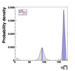
(EPS) [JPG] ρρ Only: α = [80,109]o U [158,196]o@ 95% Prob. (SM solution: α =(93 ± 10)o@ 68% Prob.)	(EPS) (JPG) ALL COMBINED: α = [7,8]o U [80,106]o U [158,176]o@ 95% Prob. (SM solution: α =(92 ± 7)o@ 68% Prob.)

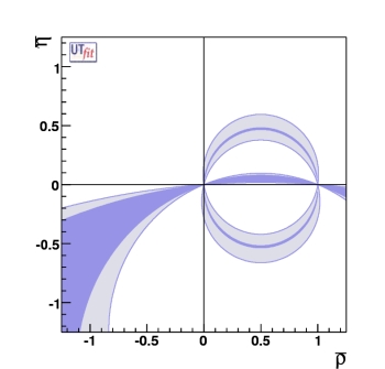
(EPS) [JPG] bound on the (ρ ; η) plane from B → ππ, B → ρρ, and and B → (ρπ)0

Observable	ππ
	Input	UTfit Output
BR(+-) (10-6)	5.2 ± 0.2	5.28 ± 0.33
BR(+0) (10-6)	5.7 ± 0.4	5.74 ± 0.42
BR(00) (10-6)	1.31 ± 0.21	1.66 ± 0.26
Observable	ρρ
	Input	UTfit Output
BR(+-) (10-6)	23.1 ± 3.3	23.4 ± 3.1
BR(+0) (10-6)	18.2 ± 3.0	17.6 ± 2.8
BR(00) (10-6)	1.2 ± 0.5	1.2 ± 0.5

(EPS) [JPG] BR+- vs BR+0 in ππ case	(EPS) [JPG] BR+- vs BR00 in ππ case
(EPS) [JPG] BR+0 vs BR00 in ππ case	(EPS) [JPG] BR+- vs BR+0 in ρρ case
(EPS) [JPG] BR+- vs BR00 in ρρ case	(EPS) [JPG] BR+0 vs BR00 in ρρ case