Determination of γ from B → D(*)K decays:
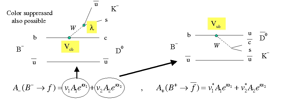
The angle γ can be measured at the B Factories comparing Vcb and Vub mediated transitions in B → D(*)K decays.
Now that the first measurements are available, it is interesting to show the available information on the value of γ.
Defining the two CP eigenstates for neutral D meson
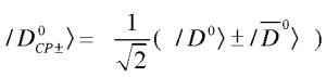
one can write B → DCP± decays as
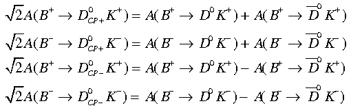
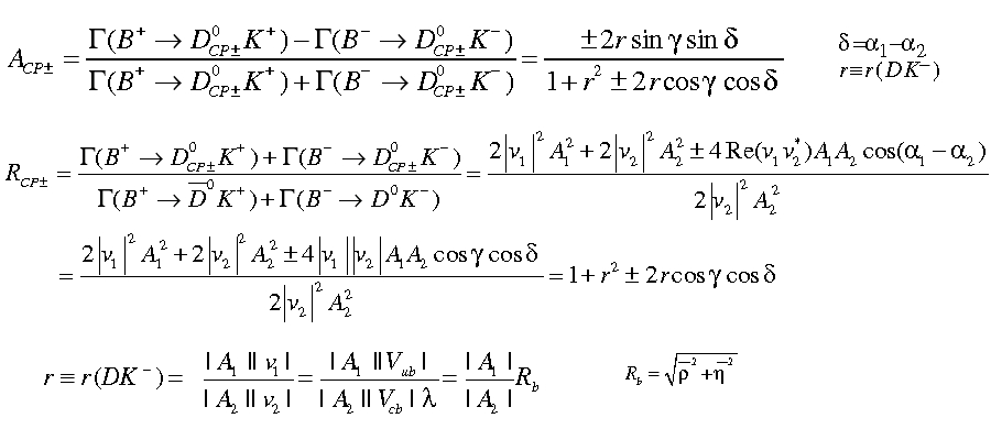
Starting from these four amplitudes, one can define four measurable quantities, which are function of γ, the difference of strong phases δ and the ratio r which is the ratio of the amplitudes corresponding to the Vub and the Vcb transitions.
Using the same formalism, one can add an other relation, considering also doubly Cabibbo suppressed decays of D meson.
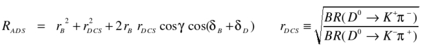
where λCab2 is the square of Cabibbo angle. This relation can be used together with the others to improve the determination of γ, even if it implies the presence of other two unknowns, rADS (in addition to r) and δD, the difference of the strong phases in the decay of the D meson. In this case CP violation appears because D0 and D0 decay into the same final state.
To access γ a new technique which make use of the D0 three-body decays, such as D0 → KS π+ π-, and a Dalitz analysis can be used (A. Giri, Yu. Grossman, A. Soffer and J. Zupan,{Phys. Rev.} D68, 054018 (2003).) The advantage of this methods is that the full sub-resonance structure of the three-body decay is considered, involving also Cabibbo allowed decays. Using this method, a GLW analysis is performed because of the interference of the CP mode (such as KS ρ (π+ π-)), an ADS analysis is also performed because of the presence of events such as K*-(KS π-) π+ from Vub and from doubly Cabibbo suppresses Vcb transitions and finally a new interference is used because of the overlap in certain regions of the Dalitz plot of decays such as K*-(KS π-) π+ and K*+(KS π+) π- Vcb and Vub mediated transitions respectively. The amplitudes for the B- and B+ can be respectively written as :
where m2- and m2+ are the squared invariant masses of the KS π- and KS π+ combinations respectively. f(m2-,m2+) is the amplitude of the D0 → KS π+ π- decay. Once the function f is fixed using a model for the D0 → KS π+ π- decay, the Dalitz distributions is thus fitted simultaneously using the expressions for the two amplitudes and rB, δB and γ can be obtained.
| DK (GLW) | ACP+ = 0.25 ± 0.07 | ACP- = -0.10 ± 0.08 | RCP+ = 1.13 ± 0.09 | RCP- = 1.06 ± 0.10 | ||
| D*K (GLW) | ACP+ = -0.12 ± 0.08 | ACP- = 0.07 ± 0.10 | RCP+ = 1.33 ± 0.12 | RCP- = 1.10 ± 0.12 | ||
| DK* (GLW) | ACP+ = 0.09 ± 0.14 | ACP- = -0.23 ± 0.22 | RCP+ = 2.17 ± 0.36 | RCP- = 1.03 ± 0.30 | ||
| DK (ADS) |
|
RADS = 0.0099 ± 0.0054 | ||||
| DK* (ADS) |
AADS = -0.34 ± 0.48 |
RADS = 0.066 ± 0.031 | ||||
| D*K (ADS) | experimental likelihood from BaBar | |||||
| DK, D->Kpipi0 (ADS) | experimental likelihood from BaBar | |||||
|
|
Dalitz Method (D → KSππ and/or D → KSKK) | BaBar [Phys.Rev.D78:034023,2008] | Belle arXiv:0803.3375v1 [hep-ex] | |||
| DK | x+= -0.087 ± 0.031 | x-= 0.097 ± 0.033 | y+= -0.038 ± 0.041 | y-= 0.101 ± 0.041 | ||
| D*K | x+= 0.136 ± 0.054 | x-= -0.084 ± 0.063 | y+= 0.101 ± 0.079 | y-= -0.100 ± 0.070 | ||
| DK* | x+= -0.109 ± 0.093 | x-= -0.057 ± 0.106 | y+= -0.056 ± 0.099 | y-= -0.165 ± 0.142 | ||
|
|
Dalitz Method (D → πππ0) | BaBar [hep-ex/0703037] | ||||
| DK | ρ+= 0.75 ± 0.13 | ρ-= 0.72 ± 0.13 | θ+= (147 ± 26)o | θ-= (173 ± 49)o | ||
| ADS (D → Kπ) |
|
RADS experimental likelihood from BaBar | ||||
| ADS (D → Kππ0) |
|
RADS experimental likelihood from BaBar | ||||
| ADS (D → Kπππ) |
|
RADS experimental likelihood from BaBar | ||||
| Dalitz (D → KSππ) | (γ,δ,rS) experimental likelihood from BaBar, arXiv:0805.2001 [hep-ex] | |||||
In the case of D → KSππ and D → KSKK Dalitz analysis for charged B decays, the quantities x± and y± are defined in terms of r, γ and δ as x± = r • cos(δ ± γ) and y± = r • sin(δ ± γ). For the systematic error coming from the model, we assume 100% correlation among the experiments. Since the model error quoted on γ is larger in the case of BaBar, we use BaBar correlation matrix for the model error when averaging the two Dalitz measurements.
Additional care has to be taken in the case of DK*: Because of the presence of a non-resonance component, all the previous formulas have to be changed in this case, replacing all the r factors appearing linearly with r • κ, being κ a factor depending in principle by the cuts applied in each analysis. The effect was found to be small by BaBar GLW analysis, which also includes a systematic contribution to it. Because of that, we identify the κ factor of the GLW analysis with that one of the Dalitz measurement, since the difference is covered by such systematic effect. The possible variation of the factor κ, evaluated from simulation studies, is taken into account in the extraction.
For D → πππ0 analysis, it was found that the use of ρ± = |(x±-x0) + i y±| and θ± = tan-1(y±/(x±-x0)) (with x0 = 0.85) represents a better choice than x± and y±, because of the reduced correlation among the variables.
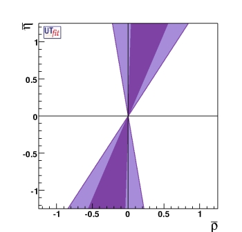
We translated these constraints in terms of a bound on (ρ ; η) plane generating r and rDCS in the range [0,1] and the strong phases in [0,2π].
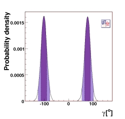
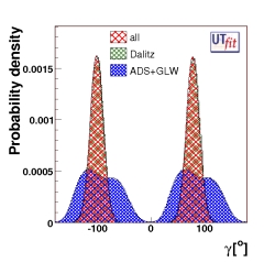
We show the distribution of γ and the corresponding effect on the (ρ ; η) plane:
|
|
||||||
|
|||||||
|
γ = 78 ± 12 ([54,102] @ 95% Prob.) γ = -102 ± 16 ([-126,-78] @ 95% Prob.) |
|||||||
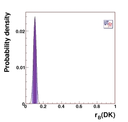
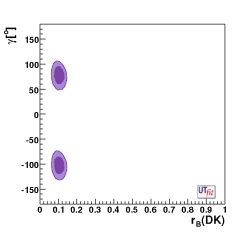
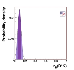
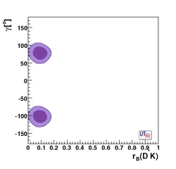
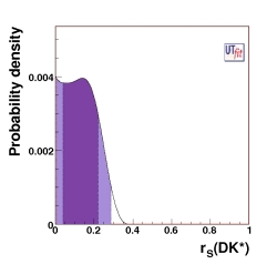
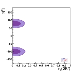
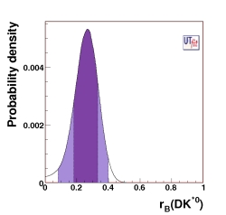
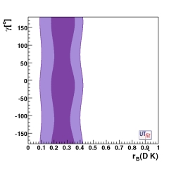
We also show the distributions of the parameters r for all the modes used (DK, D*K and DK*), together with the 2-dimensional plots of r vs γ:
|
|
||||
|
rB(DK) = 0.102 ± 0.017 ([0.069,0.133] @95% Prob.) |
|||||
|
|
||||
|
rB(D*K) = 0.089 ± 0.034 ([0.021,0.156] @95% Prob.) |
|||||
|
|
||||
|
rB(DK*) = 0.13 ± 0.09 ([0.005,0.289] @95% Prob.) |
|||||
|
|
||||
|
rB(DK*0) = 0.26 ± 0.076 ([0.081,0.397] @95% Prob.) |
|||||
We would like to thank G.Cavoto, T.Gershon, and K.Trabelsi for helping us with HFAG inputs, and F. Martinez-Vidal, G.Marchiori, N.Neri, and M. Rama for the usefull discussions on the details of BaBar measurements.
![[JPG]](gamma_deg_all.jpg)
![[JPG]](gamma_deg_overimp.jpg)
![[JPG]](CKM_fit_all.jpg)
![[JPG]](r_all.jpg)
![[JPG]](r_vs_gamma_all.jpg)
![[JPG]](rstar_all.jpg)
![[JPG]](rstar_vs_gamma_all.jpg)
![[JPG]](rkstd_all.jpg)
![[JPG]](rkstd_vs_gamma_all.jpg)
![[JPG]](rdkst0_all.jpg)
![[JPG]](rdkst0_vs_gamma_all.jpg)