
Difference: Formalism (1 vs. 14)
Revision 14
20 Sep 2011 - Main.MarcoCiuchini
Revision 13
20 Oct 2010 - Main.MarcoCiuchini
 and
and  , while
  is the weak coupling constant and
  is the field which creates the
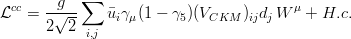
  vector boson. The CKM matrix elements are the only flavour-non-diagonal and CP-violating couplings present in the SM. In general, the CKM matrix can be parametrized using three rotation angles and one phase. The parametrization is however not unique. The standard parametrization, advocated by the PDG, uses
  in
in ![[0,\pi/2]~](/foswiki/pub/UTfit/Formalism/_MathModePlugin_9727fd85a0a15fa30280bf89f6be2378.png) and
and ![(-\pi,\pi]~](/foswiki/pub/UTfit/Formalism/_MathModePlugin_11d16201edbf57b5634f35a4edd3cafb.png) defined so that
defined so that
Revision 12
21 Jul 2010 - Main.VincenzoVagnoni
Revision 11
16 Jul 2010 - Main.VincenzoVagnoni
| Line: 1 to 1 | ||||||||
|---|---|---|---|---|---|---|---|---|
| Changed: | ||||||||
| < < |
Under construction
The Cabibbo-Kobayashi-Maskawa ( CKM) matrixis a 3x3 unitary matrix which originates from the misalignment in flavour space of the up and down components of the | |||||||
| > > |
| |||||||
| -\sin\theta_{12}\cos\theta_{23}-\cos\theta_{12}\sin\theta_{13}\sin\theta_{23}\, e^{i\delta} & \cos\theta_{12}\cos\theta_{23}-\sin\theta_{12}\sin\theta_{13}\sin\theta_{23}\, e^{i\delta} & \cos\theta_{13}\sin\theta_{23}\ | ||||||||
| Changed: | ||||||||
| < < |
\sin\theta_{12}\sin\theta_{23}-\cos\theta_{12}\sin\theta_{13}\cos\theta_{23}\, e^{i\delta} & -\cos\theta_{12}\sin\theta_{23}-\sin\theta_{12}\sin\theta_{13}\cos\theta_{23}\, e^{i\delta} & \cos\theta_{13}\cos\theta_{23}\end{array}\right)\,. The relations induced by the unitarity of the CKM matrix include six "triangular" relations, among which is referred to as the Unitarity Triangle ( UT). It can be rewritten as with  , ,  and and  , ,  are the non-trivial sides and angles of the normalized UT. The third side is the unit vector and the third angle is given by are the non-trivial sides and angles of the normalized UT. The third side is the unit vector and the third angle is given by  . The UT is determined by one complex number . The UT is determined by one complex number namely by the coordinates  in the complex plane of its only non-trivial apex (the others being (0,0) and (1,0)). Several experimental constraints can be conveniently represented on this plane and used to determine the UT, as shown in section Fit Results. We start extracting the CKM parameters from the measurements of in the complex plane of its only non-trivial apex (the others being (0,0) and (1,0)). Several experimental constraints can be conveniently represented on this plane and used to determine the UT, as shown in section Fit Results. We start extracting the CKM parameters from the measurements of  and using and using
| |||||||
| > > |
\sin\theta_{12}\sin\theta_{23}-\cos\theta_{12}\sin\theta_{13}\cos\theta_{23}\, e^{i\delta} & -\cos\theta_{12}\sin\theta_{23}-\sin\theta_{12}\sin\theta_{13}\cos\theta_{23}\, e^{i\delta} & \cos\theta_{13}\cos\theta_{23}\end{array}\right)\,.
The relations induced by the unitarity of the CKM matrix include six "triangular" relations, among which
 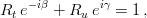  , and , are the non-trivial sides and angles of the normalized UT. The third side is the unit vector and the third angle is given by . The UT is determined by one complex number , and , are the non-trivial sides and angles of the normalized UT. The third side is the unit vector and the third angle is given by . The UT is determined by one complex number
 in the complex plane of its only non-trivial apex (the others being (0,0) and (1,0)). Several experimental constraints can be conveniently represented on this plane and used to determine the UT, as shown in section Fit Results. We start extracting the CKM parameters from the measurements of and using in the complex plane of its only non-trivial apex (the others being (0,0) and (1,0)). Several experimental constraints can be conveniently represented on this plane and used to determine the UT, as shown in section Fit Results. We start extracting the CKM parameters from the measurements of and using
| |||||||
| \cos\theta_{12}=\frac{\vert V_{ud}\vert}{\cos\theta_{13}}, & \sin\theta_{12}=\sqrt{1-\cos^2\theta_{12}},\\sin\theta_{23}=\frac{\vert V_{cb}\vert}{\cos\theta_{13}}, & \cos\theta_{23}=\sqrt{1-\sin^2\theta_{23}},\end{array} ~~\delta=2\arctan\left(\frac{1\mp\sqrt{1-(a^2-1)\tan^2\gamma}}{(a-1)\tan\gamma}\right), ~a=\frac{\cos\theta_{12}\sin\theta_{13}\sin\theta_{23}}{\sin\theta_{12}\cos\theta_{23}}. | ||||||||
| Changed: | ||||||||
| < < |
The sign  in the formula for in the formula for  corresponds to corresponds to 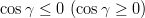 . Additional constraints, discussed in section Constraints, are then applied using the method described in section Statistical Method. Fit Results are also given in the popular Wolfenstein parametrization which allows for a transparent expansion of the CKM matrix in terms of the sine of the small Cabibbo angle . Additional constraints, discussed in section Constraints, are then applied using the method described in section Statistical Method. Fit Results are also given in the popular Wolfenstein parametrization which allows for a transparent expansion of the CKM matrix in terms of the sine of the small Cabibbo angle  . The Wolfenstain parameters . The Wolfenstain parameters  are defined by the following equations are defined by the following equations The CKM matrix can be expanded as The exact and expanded relations between the UT apex coordinates  and the Wolfenstein parameters are given by and the Wolfenstein parameters are given by At the lowest order in  , ,  and and  coincide with coincide with  and and  . . | |||||||
| > > |
The sign in the formula for corresponds to . Additional constraints, discussed in section Constraints, are then applied using the method described in section Statistical Method. Fit Results are also given in the popular Wolfenstein parametrization which allows for a transparent expansion of the CKM matrix in terms of the sine of the small Cabibbo angle . The Wolfenstain parameters are defined by the following equations
  and the Wolfenstein parameters are given by and the Wolfenstein parameters are given by
 , and coincide with and . , and coincide with and . | |||||||

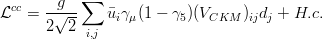
 quark doublet of the Standard Model ( SM). In the quark mass eigenstate basis, the CKM matrix appears in the SM charged-current interaction Lagrangian
Revision 10
29 Jun 2010 - Main.MarcoCiuchini
| Line: 1 to 1 | ||||||||
|---|---|---|---|---|---|---|---|---|
| Under construction | ||||||||
| Changed: | ||||||||
| < < |
The Cabibbo-Kobayashi-Maskawa ( CKM) matrixis a 3x3 unitary matrix which originates from the misalignment in flavour space of the up and down components of the | |||||||
| > > |
The Cabibbo-Kobayashi-Maskawa ( CKM) matrixis a 3x3 unitary matrix which originates from the misalignment in flavour space of the up and down components of the | |||||||
-\sin\theta_{12}\cos\theta_{23}-\cos\theta_{12}\sin\theta_{13}\sin\theta_{23}\, e^{i\delta} & \cos\theta_{12}\cos\theta_{23}-\sin\theta_{12}\sin\theta_{13}\sin\theta_{23}\, e^{i\delta} & \cos\theta_{13}\sin\theta_{23}\\sin\theta_{12}\sin\theta_{23}-\cos\theta_{12}\sin\theta_{13}\cos\theta_{23}\, e^{i\delta} & -\cos\theta_{12}\sin\theta_{23}-\sin\theta_{12}\sin\theta_{13}\cos\theta_{23}\, e^{i\delta} & \cos\theta_{13}\cos\theta_{23}\end{array}\right)\,. The relations induced by the unitarity of the CKM matrix include six "triangular" relations, among which is referred to as the Unitarity Triangle ( UT). It can be rewritten as with , and , are the non-trivial sides and angles of the normalized UT. The third side is the unit vector and the third angle is given by . The UT is determined by one complex number namely by the coordinates in the complex plane of its only non-trivial apex (the others being (0,0) and (1,0)). Several experimental constraints can be conveniently represented on this plane and used to determine the UT, as shown in section Fit Results. We start extracting the CKM parameters from the measurements of and using
| ||||||||
| Changed: | ||||||||
| < < |
The sign in the formula for corresponds to . Additional constraints, discussed in section Constraints, are then applied using the method described in section Statistical Method. Fit Results are also given in the popular Wolfenstein parametrization which allows for a transparent expansion of the CKM matrix in terms of the sine of the small Cabibbo angle . The Wolfenstain parameters are defined by the following equations The CKM matrix can be expanded as The exact and expanded relations between and the Wolfenstein parameters are given by At the lowest order in , and coincide with the UT apex coordinates and . | |||||||
| > > |
The sign in the formula for corresponds to . Additional constraints, discussed in section Constraints, are then applied using the method described in section Statistical Method. Fit Results are also given in the popular Wolfenstein parametrization which allows for a transparent expansion of the CKM matrix in terms of the sine of the small Cabibbo angle . The Wolfenstain parameters are defined by the following equations The CKM matrix can be expanded as The exact and expanded relations between the UT apex coordinates and the Wolfenstein parameters are given by At the lowest order in , and coincide with and . | |||||||
Revision 9
29 Jun 2010 - Main.AdrianBevan
| Line: 1 to 1 | ||||||||
|---|---|---|---|---|---|---|---|---|
| Under construction | ||||||||
| Changed: | ||||||||
| < < |
The Cabibbo-Kobayashi-Maskawa ( CKM) matrixis a 3x3 unitary matrix which originates from the disalignment in flavour space of the up and down components of the | |||||||
| > > |
The Cabibbo-Kobayashi-Maskawa ( CKM) matrixis a 3x3 unitary matrix which originates from the misalignment in flavour space of the up and down components of the | |||||||
-\sin\theta_{12}\cos\theta_{23}-\cos\theta_{12}\sin\theta_{13}\sin\theta_{23}\, e^{i\delta} & \cos\theta_{12}\cos\theta_{23}-\sin\theta_{12}\sin\theta_{13}\sin\theta_{23}\, e^{i\delta} & \cos\theta_{13}\sin\theta_{23}\\sin\theta_{12}\sin\theta_{23}-\cos\theta_{12}\sin\theta_{13}\cos\theta_{23}\, e^{i\delta} & -\cos\theta_{12}\sin\theta_{23}-\sin\theta_{12}\sin\theta_{13}\cos\theta_{23}\, e^{i\delta} & \cos\theta_{13}\cos\theta_{23}\end{array}\right)\,. The relations induced by the unitarity of the CKM matrix include six "triangular" relations, among which is referred to as the Unitarity Triangle ( UT). It can be rewritten as with , and , are the non-trivial sides and angles of the normalized UT. The third side is the unit vector and the third angle is given by . The UT is determined by one complex number namely by the coordinates in the complex plane of its only non-trivial apex (the others being (0,0) and (1,0)). Several experimental constraints can be conveniently represented on this plane and used to determine the UT, as shown in section Fit Results. We start extracting the CKM parameters from the measurements of and using
| ||||||||
Revision 8
28 Jun 2010 - Main.MarcoCiuchini
| Line: 1 to 1 | ||||||||
|---|---|---|---|---|---|---|---|---|
Under construction
The Cabibbo-Kobayashi-Maskawa ( CKM) matrixis a 3x3 unitary matrix which originates from the disalignment in flavour space of the up and down components of the | ||||||||
| Line: 7 to 7 | ||||||||
| \sin\theta_{23}=\frac{\vert V_{cb}\vert}{\cos\theta_{13}}, & \cos\theta_{23}=\sqrt{1-\sin^2\theta_{23}},\end{array} ~~\delta=2\arctan\left(\frac{1\mp\sqrt{1-(a^2-1)\tan^2\gamma}}{(a-1)\tan\gamma}\right), ~a=\frac{\cos\theta_{12}\sin\theta_{13}\sin\theta_{23}}{\sin\theta_{12}\cos\theta_{23}}. | ||||||||
| Changed: | ||||||||
| < < |
The sign in the formula for corresponds to . Additional constraints, discussed in section Constraints, are then applied using the method described in section Statistical Method. Fit Results are also given in the popular Wolfenstein parametrization which allows for a transparent expansion of the CKM matrix in terms of the small Cabibbo angle . The Wolfenstain parameters are defined by the following equations At the first order,  is the Cabibbo angle and and coincide with the UT coordinates and . The exact relation between is the Cabibbo angle and and coincide with the UT coordinates and . The exact relation between  and is given by and is given by </latex></latex> | |||||||
| > > |
The sign in the formula for corresponds to . Additional constraints, discussed in section Constraints, are then applied using the method described in section Statistical Method. Fit Results are also given in the popular Wolfenstein parametrization which allows for a transparent expansion of the CKM matrix in terms of the sine of the small Cabibbo angle . The Wolfenstain parameters are defined by the following equations The CKM matrix can be expanded as The exact and expanded relations between and the Wolfenstein parameters are given by At the lowest order in , and coincide with the UT apex coordinates and . | |||||||
Revision 7
28 Jun 2010 - Main.MarcoCiuchini
| Line: 1 to 1 | ||||||||
|---|---|---|---|---|---|---|---|---|
| Under construction | ||||||||
| Changed: | ||||||||
| < < |
The Cabibbo-Kobayashi-Maskawa ( CKM) matrixis a 3x3 unitary matrix which originates from the disalignment in flavour space of the up and down components of the | |||||||
| > > |
The Cabibbo-Kobayashi-Maskawa ( CKM) matrixis a 3x3 unitary matrix which originates from the disalignment in flavour space of the up and down components of the | |||||||
| -\sin\theta_{12}\cos\theta_{23}-\cos\theta_{12}\sin\theta_{13}\sin\theta_{23}\, e^{i\delta} & \cos\theta_{12}\cos\theta_{23}-\sin\theta_{12}\sin\theta_{13}\sin\theta_{23}\, e^{i\delta} & \cos\theta_{13}\sin\theta_{23}\ | ||||||||
| Changed: | ||||||||
| < < |
\sin\theta_{12}\sin\theta_{23}-\cos\theta_{12}\sin\theta_{13}\cos\theta_{23}\, e^{i\delta} & -\cos\theta_{12}\sin\theta_{23}-\sin\theta_{12}\sin\theta_{13}\cos\theta_{23}\, e^{i\delta} & \cos\theta_{13}\cos\theta_{23}\end{array}\right)\,. We start extracting the CKM parameters from the measurements of 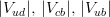 and and  using using
| |||||||
| > > |
\sin\theta_{12}\sin\theta_{23}-\cos\theta_{12}\sin\theta_{13}\cos\theta_{23}\, e^{i\delta} & -\cos\theta_{12}\sin\theta_{23}-\sin\theta_{12}\sin\theta_{13}\cos\theta_{23}\, e^{i\delta} & \cos\theta_{13}\cos\theta_{23}\end{array}\right)\,. The relations induced by the unitarity of the CKM matrix include six "triangular" relations, among which is referred to as the Unitarity Triangle ( UT). It can be rewritten as with , and , are the non-trivial sides and angles of the normalized UT. The third side is the unit vector and the third angle is given by . The UT is determined by one complex number namely by the coordinates in the complex plane of its only non-trivial apex (the others being (0,0) and (1,0)). Several experimental constraints can be conveniently represented on this plane and used to determine the UT, as shown in section Fit Results. We start extracting the CKM parameters from the measurements of and using
| |||||||
| \cos\theta_{12}=\frac{\vert V_{ud}\vert}{\cos\theta_{13}}, & \sin\theta_{12}=\sqrt{1-\cos^2\theta_{12}},\\sin\theta_{23}=\frac{\vert V_{cb}\vert}{\cos\theta_{13}}, & \cos\theta_{23}=\sqrt{1-\sin^2\theta_{23}},\end{array} ~~\delta=2\arctan\left(\frac{1\mp\sqrt{1-(a^2-1)\tan^2\gamma}}{(a-1)\tan\gamma}\right), ~a=\frac{\cos\theta_{12}\sin\theta_{13}\sin\theta_{23}}{\sin\theta_{12}\cos\theta_{23}}. | ||||||||
| Changed: | ||||||||
| < < |
The sign  in the formula for in the formula for  corresponds to corresponds to  . Additional constraints are then applied using the method described in the section Statistical Method. Results are also given in the popular Wolfenstein parametrization which allows for a transparent expansion of the CKM matrix in terms of the small Cabibbo angle . The Wolfenstain parameters . Additional constraints are then applied using the method described in the section Statistical Method. Results are also given in the popular Wolfenstein parametrization which allows for a transparent expansion of the CKM matrix in terms of the small Cabibbo angle . The Wolfenstain parameters  are defined by the following equations are defined by the following equations The relations induced by the unitarity of the CKM matrix include six "triangular" relations, among which is referred to as the Unitarity Triangle ( UT). It can be rewritten as with | |||||||
| > > |
The sign in the formula for corresponds to . Additional constraints, discussed in section Constraints, are then applied using the method described in section Statistical Method. Fit Results are also given in the popular Wolfenstein parametrization which allows for a transparent expansion of the CKM matrix in terms of the small Cabibbo angle . The Wolfenstain parameters are defined by the following equations At the first order, is the Cabibbo angle and and coincide with the UT coordinates and . The exact relation between and is given by </latex></latex> | |||||||
 quark doublet of the Standard Model ( SM). In the quark mass eigenstate basis, the CKM matrix appears in the SM charged-current interaction Lagrangian
  and
and  is the weak coupling constant and
  is the field which creates the
  vector boson. The CKM matrix elements are the only flavour- and CP-violating couplings present in the SM. In general, the CKM matrix can be parametrized using three rotation angles and one phase. The parametrization is however not unique. The standard parametrization, advocated by the PDG, uses
  in
in ![[0,\pi/2]](/foswiki/pub/UTfit/Formalism/_MathModePlugin_73e40ef7b3aa437628df055b85658888.png) and
and ![(-\pi,\pi]](/foswiki/pub/UTfit/Formalism/_MathModePlugin_5274755a90f82e76034c6660a7fee565.png) defined so that
defined so that
Revision 6
17 Jun 2010 - Main.AchilleStocchi
| Line: 1 to 1 | ||||||||
|---|---|---|---|---|---|---|---|---|
Under construction
The Cabibbo-Kobayashi-Maskawa ( CKM) matrixis a 3x3 unitary matrix which originates from the disalignment in flavour space of the up and down components of the | ||||||||
Revision 5
17 Jun 2010 - Main.MarcoCiuchini
| Line: 1 to 1 | ||||||||
|---|---|---|---|---|---|---|---|---|
Under construction
The Cabibbo-Kobayashi-Maskawa ( CKM) matrixis a 3x3 unitary matrix which originates from the disalignment in flavour space of the up and down components of the | ||||||||
| Line: 7 to 7 | ||||||||
| \sin\theta_{23}=\frac{\vert V_{cb}\vert}{\cos\theta_{13}}, & \cos\theta_{23}=\sqrt{1-\sin^2\theta_{23}},\end{array} ~~\delta=2\arctan\left(\frac{1\mp\sqrt{1-(a^2-1)\tan^2\gamma}}{(a-1)\tan\gamma}\right), ~a=\frac{\cos\theta_{12}\sin\theta_{13}\sin\theta_{23}}{\sin\theta_{12}\cos\theta_{23}}. | ||||||||
| Changed: | ||||||||
| < < |
The sign in the formula for corresponds to 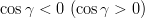 . Additional constraints are then applied using the method described in the section Statistical Method. Results are also given in the popular Wolfenstein parametrization which allows for a transparent expansion of the CKM matrix in terms of the small Cabibbo angle . The Wolfenstain parameters are defined by the following equations . Additional constraints are then applied using the method described in the section Statistical Method. Results are also given in the popular Wolfenstein parametrization which allows for a transparent expansion of the CKM matrix in terms of the small Cabibbo angle . The Wolfenstain parameters are defined by the following equations The relations induced by the unitarity of the CKM matrix include six "triangular" relations, among which is referred to as the Unitarity Triangle ( UT). It can be rewritten as with | |||||||
| > > |
The sign in the formula for corresponds to . Additional constraints are then applied using the method described in the section Statistical Method. Results are also given in the popular Wolfenstein parametrization which allows for a transparent expansion of the CKM matrix in terms of the small Cabibbo angle . The Wolfenstain parameters are defined by the following equations The relations induced by the unitarity of the CKM matrix include six "triangular" relations, among which is referred to as the Unitarity Triangle ( UT). It can be rewritten as with | |||||||
Revision 4
16 Jun 2010 - Main.MarcoCiuchini
| Line: 1 to 1 | ||||||||
|---|---|---|---|---|---|---|---|---|
| Under construction | ||||||||
| Changed: | ||||||||
| < < |
The Cabibbo-Kobayashi-Maskawa ( CKM) matrixis a 3x3 unitary matrix which originates from the disalignment in flavour space of the up and down components of the | |||||||
| > > |
The Cabibbo-Kobayashi-Maskawa ( CKM) matrixis a 3x3 unitary matrix which originates from the disalignment in flavour space of the up and down components of the | |||||||
| \cos\theta_{12}=\frac{\vert V_{ud}\vert}{\cos\theta_{13}}, & \sin\theta_{12}=\sqrt{1-\cos^2\theta_{12}},\\sin\theta_{23}=\frac{\vert V_{cb}\vert}{\cos\theta_{13}}, & \cos\theta_{23}=\sqrt{1-\sin^2\theta_{23}},\end{array} ~~\delta=2\arctan\left(\frac{1\mp\sqrt{1-(a^2-1)\tan^2\gamma}}{(a-1)\tan\gamma}\right), ~a=\frac{\cos\theta_{12}\sin\theta_{13}\sin\theta_{23}}{\sin\theta_{12}\cos\theta_{23}}. | ||||||||
| Changed: | ||||||||
| < < |
The sign in the formula for corresponds to . | |||||||
| > > |
The sign in the formula for corresponds to . Additional constraints are then applied using the method described in the section Statistical Method. Results are also given in the popular Wolfenstein parametrization which allows for a transparent expansion of the CKM matrix in terms of the small Cabibbo angle . The Wolfenstain parameters are defined by the following equations The relations induced by the unitarity of the CKM matrix include six "triangular" relations, among which is referred to as the Unitarity Triangle ( UT). It can be rewritten as with | |||||||
 in
in 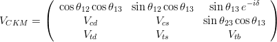

Revision 3
11 Jun 2010 - Main.MarcoCiuchini
| Line: 1 to 1 | ||||||||
|---|---|---|---|---|---|---|---|---|
| Under construction | ||||||||
| Changed: | ||||||||
| < < |
| |||||||
| > > |
The Cabibbo-Kobayashi-Maskawa ( CKM) matrixis a 3x3 unitary matrix which originates from the disalignment in flavour space of the up and down components of the | |||||||

Revision 2
18 May 2010 - Main.MarcoCiuchini
| Line: 1 to 1 | ||||||||
|---|---|---|---|---|---|---|---|---|
| Under construction | ||||||||
| Added: | ||||||||
| > > |
| |||||||
View topic | History: r14 < r13 < r12 < r11 | More topic actions...
Powered by
 Ideas, requests, problems regarding this web site? Send feedback